We use three simple estimators from the scikit-learn library (add links)

• SVC with the Linear kernel
• SVC with the Radial Basis Function kernel
• K Nearest Neighbor

Support Vector Classifiers

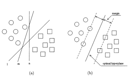
Support vector classification is a machine learning technique where data points are represented as vectors, often in a high-dimensional space, with each dimension corresponding to a different feature or attribute. The algorithm works by finding a decision boundary (typically a hyperplane) that optimally separates different classes of data points in this feature space.

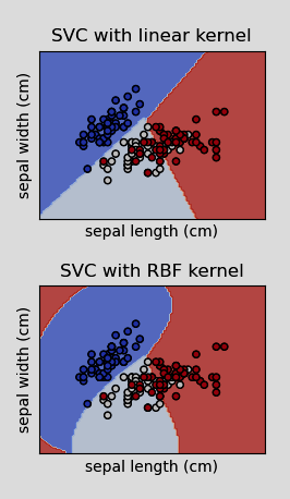
SVC with linear kernel vs SVC with Radial Basis Function kernel

The primary difference between using a linear and radial basis function kernel is that linear kernels create a decision boundary that is a straight line or in the higher dimensions a flat hyperplane.

A radial basis function on the other hand can create a curved line/hyperplane.

• In "Content-Based Audio Classification and Retrieval by Support Vector Machine", the authors outline a set of kernel functions used to map the linear input space of the SVM to a multidimensional feature space. In particular they found through experimentation that using an exponential radial basis function (ERBF) resulted in the best model performance (Guo & Li, 2003).
• include any settings for SVC/Linear SVC (ie, balanced etc)

K Nearest Neighbor (KNN)

KNN is a simple algorithm used for classification assumes similar items are closer together in the feature space. It doesn't generalize like SVCs. With the SVC models we train them on a set of data, then we get a set of model weights that we can use to get a prediction back.

Instead with KNN, when we pass an example:

• It computes the "distance" to the examples in our "training" set. Typically, this is the Euclidean distance between each data point in our example feature vector and the corresponding point in each of the rest of the feature vectors in the set.
• It finds the n (a number chosen by the user) closest examples in the set and gives each one a "vote," which simply consists of the label attacvhed to that example.
• The sample we want a prediction for is classified according to whichever class has the majority of votes.
• For example: Imagine we want to classify the RAVDESS samples according to actor sex using KNN. We will set the number of neighbors (n) to 5.
• After passing our sample to KNN it calculates the distance from our sample to the examples in the "training" set.
• The algorithm then looks at the labels of the 5 closest examples.
• From those 5 examples, if 3 are female and 2 are male, our sample will be classified as female.
• Conversely, if 2 are female and 3 are male, our sample will be classified as male.

Testing and Performance Metrics

While there are many ways of evaluating estimator performance, we will keep it simple and direct focusing on a confusion matrix and three metrics derived from it: recall, precision, and accuracy.

Returning to the example of actor sex, assume we've trained our model to identify female actors.

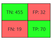
A confusion matrix, like the one below, simply tells us how many:

• True Positives (TP = 70): The actor is female. The model correctly identifies the actor as female.
• False Positives (FP = 32): The actor is male. The model incorrectly identifies the actor as female.
• True Negatives (TN = 455): The actor is male. The model correctly identifies the actor as male.
• False Negatives (FN = 19): The actor is female. The model incorrectly identifies the actor as male.

We then use those values to derive:

• Recall = TP / (TP + FN) = 0.78
  • Measures the ratio of positive classes the model correctly identifies.
• Precision = TP / (TP + FP) = 0.69
  • Measures how often the model is correct when identifying the positive class.
• Accuracy = (TP + TN) / (TP + TN + FP + FN) = 0.91
  • Measures the ratio of examples the model correctly identified.

Next:

Continue to the interactive class selector.