Representing digital audio
Waveform
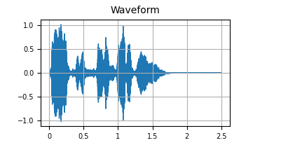
Digital audio is typically represented as a floating-point array of amplitudes with attached metadata (in the form of a sample rate) indicating how fast an application should read the file. That is, a digital audio file describes amplitude over time. This is particularly useful if you want to send a sequence of voltages to a speaker, but less so for language processing. Though some models like Wav2Vec2 do initially ingest audio this way.
Consider that each 2.5 second, 16kHz RAVDESS sample consists of 2.5 x 16,000 = 40,000 data points.
Why we transform
The transformations represent the audio in a way that is more inline with our perception
- We perceive sound along a number of dimensions, not just amplitude.
- Frequency and its perceptual complement pitch is especially important.
- The combination of frequency and amplitude over time also gives us important information about the timbre, or the quality of the sound. This is especially important for speech tasks as we'll see later.
- As pitch, volume and timbre are how we as humans describe sonic phenomena, it makes intuitive sense that when training or inferring from a model that we'd be looking to characterize our examples using those aspects of sound.
- We represent amplitude and frequency linearly in the digital domain.
- But we perceive loudness along a log scale and pitch along a "Mel" scale.
- As part of the transformation process, we scale the data to match our perception.
We are compressing the information
- In extracting features, we ideally amplify those characteristics we are interested in and attenuate those we are not. In other words, we improve signal to noise.
- This has the additional benefit of making training and inference faster as we're working with less data.
Transformations
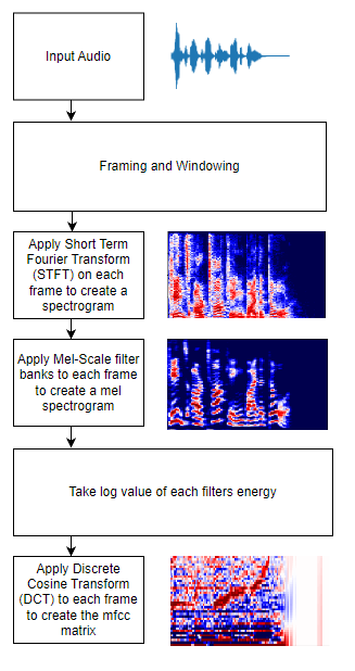
Process Overview
STFT: Short-Time Fourier Transform
The framing and windowing process divides the audio sample into many smaller, overlapping audio slices, typically 20-30ms in length. The windowing aspect controls the overlap between adjacent frames, often ~ 10ms.
Next a Short-Time Fourier Transform (STFT) is performed on each frame. The STFT changes a signal's time domain to its frequency domain. It does this by dividing each frame into a number of frequency bins and then calculating the power spectrum for each bin in each frame.
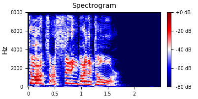
This process produces a spectrogram.
- The y-axis is frequency.
- The x-axis is time.
- The z-axis is power at that frequency at that time.
A spectrogram of the above waveform, when calculated with an fft size of 512 and 257 frequency bins gives us a matrix of size 257 x 108. Which is 27,756 data points.
For an excellent introduction to Fourier Transforms see this 3Blue1Brown video.
Now we have frequency and amplitude info over time, but we can scale and process further for more information and less noise.
Mel Spectrogram
At lower frequencies humans perceive the distance between intervals as larger than at higher frequencies.
- For example we hear the interval 440hz, 660hz, a difference of 220Hz as a perfect fifth.
- The interval from 3951hz to 4186hz, a difference of 235hz is perceived as a half step, a much smaller interval!
- And for those lucky enough to still have their hearing up there, there's little perceivable difference between 14220 and 14220.
To account for this we apply a set of "mel" filters to the STFT/spectrogram where the width of the filters corresponds to our perception of pitch.
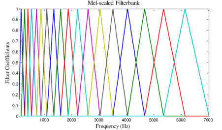
- Then we simply sum up the power in each filter.
- Our resulting matrix still has frequency on the y-axis and time on the x-axis.
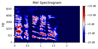
Our mel spectrogram, even using a generous 128 filters, has dimensions of 128 x 108, or 13,824 data points per example, making it roughly 1/3 the size of our original waveform.
MFCC: Mel Frequency Cepstral Coefficients
The final piece of our feature extraction process is transforming the mel spectrograms into mfcc matrices. Similarly to how we used the Fourier transform to move our audio into the frequency domain, we use a discrete cosine transform (DCT) to move our mel spectrogram into what I sometimes think of as the timbral domain.
MFCCs allow us to separate out the phonemes from the glottal pulse.
- Glottal pulse - the broad spectrum noise generated by our vocal folds.
- Phonemes - the sounds resulting from the use of our mouth (teeth, tongues, lips, etc) to filter the glottal pulse.
- Phonemes represent the spectral envelope of speech sound. This is often where the "information" is represented: words, emotions, etc. That is to say, we use phonemes to construct our language.
- By separating out the phonemes, we can train our model specifically on the information we are interested in while ignoring the information we are not.
Power scaling
- As with pitch, our perception of amplitude (aka loudness) differs from the digital representation of loudness. We perceive loudness along a log scale.
- So, our first step in deriving our MFCC is to take the log of each frequency/time value from the Mel Spectrogram.
Discrete Cosine Transform (DCT)
- Like an FFT, DCT expresses signals as the sum of of sinusoids with different amplitudes and frequencies, but DCT only uses cosine functions and use real numbers.
- We apply the DCT to each frame of the mel spectrogram.
- Now we have the MFCC bin on the y-axis with time still on the x-axis.
- We can think of the coefficient values as representing how similar the mel spectrogram is to one of the cosine shapes.
- Most of the spectral envelope will be captured in the first 12-13 coefficients.
- The higher coefficients encode the glottal pulse.
- MFCC 0 is just the overall loudness.
- FluCoMa has a great interactive tool for exploring mfccs and how they are dervived.
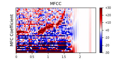
If we use 20 MFCCs, then our data has dimensions of 20 x 108, for 2,160 data points. That's only 5.4% the size of our original sample!
Next:
Continue to the interactive feature extractor.